Integrated use of webpages, spreadsheets and textbooks to create an interactive learning environment in higher mathematics.

Freyr Thorarinsson, Ph.D.
freyr@verslo.is
Commercial College of Iceland
Ofanleiti 1, 103 Reykjavik


Abstract: A new kind of teaching materials, which integrate the use of webpages, spreadsheets and textbooks, has been devolped for courses in higher mathematics including differential equations, matrix calculations and statistics. The textbooks explain the subject with an emphasis on computer applications and refer any lengthy calculations to Excel spreadsheets. The webpages cover the same material from a more encyclopedic point of view and include live links to sample spreadsheets for all problems discussed. This approach allow the teacher to focus on the concepts rather than techniques, introduces the students to realistic applications of the mathematical ideas and makes it possible to use large datasets in student exercises.

A new kind of teaching material in mathematics for the last year of secondary school has been developed and used for a few years at the Commercial College in Iceland. This includes textbooks, webpages and spreadsheet examples designed to support each other as complementary and referential material. The subjects dealt with include ordinary differential equations and their numerical solutions, matrix calculations, data analysis and statistics.
The textbooks explain mathematical ideas without proofing a lot of theorems, and put an emphasis on computer applications, in particular on the way calculations are carried out in Excel spreadsheets. In some ways the textbooks can be viewed as a quick guide to the subject. The textbooks are accompanied by webpages, where the same material is treated with a different perspective. The webpages cover e.g. historical background material, definitions and translations of words, detailed proofs of important theorems and alternative explanations of mathematical ideas. The web, by its nature, keeps growing and expanding and it is kept available in a compressed format for the students to download and set up on their own computers. The example spreadsheets are explained and referred to in the textbooks and included in the webpages in such a way that when the student clicks on an example, Excel is activated and the student can manipulate the spreadsheet, change the data or the parameters in an equation and observe the effects on the resulting calculations. This allows the discussion of cases in the to be limited to small examples for clarity, and at the same time provides substancial examples for study and exercises.
The integration of textbook, webpages and spreadsheets lets the textbook focus on the concepts rather than techniques or proofs, while the use of spreadsheets as a tool to carry out all calculations introduces the students to realistic applications of the mathematical ideas. The encyclopedic and dynamic nature of the web offers the teacher an opportunity to extend the material in any direction and tailor it to the needs of various student groups without the need for a new textbook.
Figures 1, 2 and 3 are are screenshots which demonstrate the use of Excel spreadsheets for various mathematical applications and student exercises. Figure 1 shows a closed form solution to a linear and homogenous differential equation with constant coefficients. The solution is controlled by the constants of the equation and the initial conditions, all of which can be adjusted to study their influence on the solution. Figure 2 shows a family of curves that satisfy a first order differential equation. All the parameters defining the family are adjustable and any change in them immediately brings out a new graph. Figure 3 shows how a time series is analysed by separating it into a linear trend and periodic oscillations.

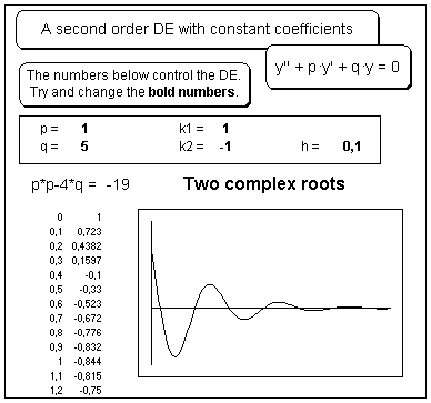
Figure 1. A 2nd order DE solution.
The general solution of a linear and homogenous differential equation with constant coefficients, y'' + py + qy = 0, can be programmed in Excel, given some values for the DE constants p and q, as well as the constants k1 and k2 which define the initial conditions.
A part of such a spreadsheet is shown in the picture. The constants defining the solution of the equation are displayed in bold font on the framed area ("the control panel") and the students can change their values at will.
The sign of the characteristic equation p·p - 4·q, shown below the control panel, decides if the DE has real or complex roots. A negative value gives rise to two complex roots and a solution of damped oscillations.
The trace of the solution is calculated in steps of h = 0.1 in the spreadsheet columns on the bottom left in the picture and displayed on the graph to the right. The student can adjust the parameters on the control panel and instantanously observe the graphical behaviour of the solution. This helps develop an intuitative feeling for the dynamic interplay between the parameters of the equation and its solution.

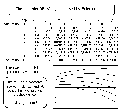
Figure 2. A DE numerical solution.
A family of solutions for a general 2nd order differential equation is shown on the picture.
The initial conditions for the equation are put in the top row in the table on the spreadsheet, the many y-values separated by an arbitrary constant dy. The numerical formula defining the next step of the solution are put in the second row, and that row is then copied as many times as needed to trace out the whole solution.
The student can vary the initial conditions or adjust the step size and observe the effects on a graph of the numerical solution. If an exact solution is available, it might also be included on the graph to display the errors in the numerical solution.

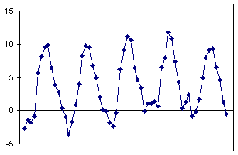
Figure 3.a. Time series analysis.
The data on the graph show the average monthly temperatures at a weather station in Iceland over a five year period. The all the following data analysis is carried out by mathematical functions frovided in Excel and its add-in Analysis Toolpack.
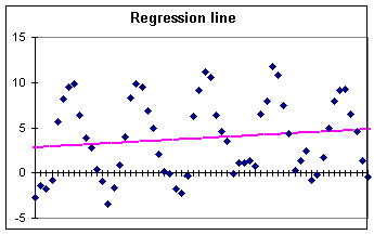
Figure 3.b. Trend analysis.
A variety of trend lines can be automatically fitted to the data and the resulting mathematical function can also be displayed on the chart. A linear trend has been fitted to the data in the figure and the line parameters (not shown) used to calculate the trend values.
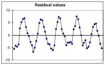
Figure 3.c. Residual values.
The trend values from 3.b have now been subtracted from the original data, leaving residual values fit for periodic analysis. A weak second order trend with a peak in the middle of the graph is visible here and its reality might be discussed with the students.
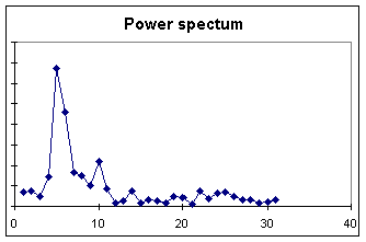
Figure 3.d. A power spectum. Excel supports the calculation of a discrete Fourier transform of the data. This material, however, is only suitable for the more mathematically advanced students and is not discussed in the textbook, but is included on the webpages.
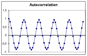
Figure 3.e. Autocorrelation.
An easier way to detect periodicity in a signal is to do calculate the autocorrelation for the series. Since the temperature data is dominated by annual oscillations, the autocorrelation graph is very regular. Less regular data, for example the classic sunspot data also included on the webpages, shows a much more irregular autocorrelation.